


 CC BY
CC BY 29
29
References:
1. Bruk V M., Nikolaev V. I. System Engineering: methods and applications. - St.-Petersburg: Mashinostroenie, 1985.
2. Scittner Lars. General Systems Theory. Ideas and applications. - World Scientific Publishing Co. - 2001.
3. Sadowski V. N. Foundations of General Systems Theory. - M.: Nauka, 1974.
4. Tokarev M. V System approach to design information systems//Conf.: "System analysis and information technology" V 2. - Cheliabinsk, Russia, 2011. - P. 75-77.
5. Tokarev M. V On the definition of General Systems Theory//European Science Review. - March-April 2014. - P. 144-147.
6. [Electronic resource]. - Available from: http://systemotechnica.ucoz.com/load/nashi_publikacii/publikacii_po_sistemotekh-nike/universalnaja_metodika_proektirovanija_informacionnykh_sistem_umasd/12-1-0-96.
7. [Electronic resource]. - Available from: http://www. vocabulary.com
Khujaev Jamol Ismatullayevich, senior researcher, Center for the development of software and hardware-program complexes at Tashkent University of Information Technologies E-mail: jamolhoja@mail.ru
Synthesis of the Fourier representation of daily changes in ambient temperature on the basis of empirical data
Abstract: A way of representing the daily changes in temperature in the lower layers of the earth's atmosphere is offered in the paper. On the basis of known dimensionless empirical data on temperature changes, the primary form of the Fourier series is constructed. To match the extreme points and the values of the final temperature in the form of the Fourier series with the newly obtained experimental data, the boundaries of links are displaced and linear deformation of curves is performed. The method can be generalized for the three- and multilink conversions of various periodic functions.
Keywords: daily temperature change, Fourier representation, approximation, empirical data.
The ambient temperature is involved in mathematical modeling and solution of many practical problems. Its adequate mathematical expression contributes obtaining the exact solutions of the problems, and make better decisions on technological processes.
At large distances from the surface of the earth the temperature has a certain static pattern [1, 233]. In certain depth (10 m. or more), the temperature of the soil, if it is not anomalous zone, has a constant value, which increases with increasing depth according to a temperature gradient of the terrain. Despite this, in practice, all geographical latitudes of the Earth have their own variable average annual temperature conditions.
Thus, at the lower boundary layer of the atmosphere and in the upper layers of the earth there are significant changes in temperature. These temperature changes are primarily related to daily and annual positions of the earth relative to the sun, the latitude and the location of the area relative to global sea level and weather conditions.
b 1,0 0,8 0,6 0,4 0,2 0 -0,2 -0,4 -0,6 -0,8 -1,0
Daily changes in temperature can be noticed in shallow depths (0.2-1.0 m.) of earth's surface, and the effect of the annual change is felt up to a depth of10 m., and in some places up to 40 m. We cannot talk regarding the temperature of the lower layer of the atmosphere such strictly, because it is "turbulent "and, in general, it depends on prehistoric processes, solar radiation and other factors. Therefore, experts prefer to use the average parameters of the atmospheric temperature.
In this work we focus on the daily temperature change in the lower parts of the atmosphere regarding to medium latitudes. The latitudes, where Uzbekistan is located ( 37°11' — 45036') is peculiar to the subtropical (the southern regions) and continental (northern and middle areas) climates. Significant diurnal temperature fluctuations, peculiar to continental climate is noticeable from year to year due to the drying process of Aral Sea.
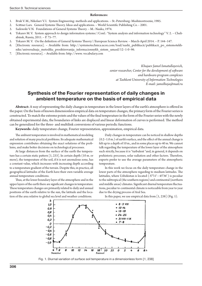
In this paper, we use empirical data from [1, 238] (Fig. 1).
: r / _ • 8~3 VIII í\ - /J-/4 -18-19 A a 24-25 o 31VIII-1IX \t * 7-8
: J K ) 1 1 1 I I 1 I 1 I 1 I 1
4 I 6 8
Sunrise
10
12 /4 16 181 20 22
Sunset
6 8h
Fig. 1. Diurnal variation of surface soil temperature in a dimensionless form [1, 238]
As can be seen from the figure, the curve of the daily changes in temperature consists of three specific units. With sunrise the temperature starts to rise, depending on the increase in the height of the sun and reduce the length of the path of the sun rays through the atmospheric layer. It reaches its peak in the afternoon, when the path of sunrays through the atmospheric layer begins to grow and the height of the sun decreases. Further, the temperature falls with certain intensity. With the onset of the dark part of the day the temperature continues to decrease, but more slowly than in the second unit. In the morning, the temperature begins to rise again, etc.
The data in the figure refer to the end of summer and beginning of autumn. They summarize the results of a series of field observations, which are presented in the segment [-1; +1] .The graph represents the variation of temperature, but not the real interval. Moreover, in the summer the light part of day is longer, and in the winter — it is shorter than the period given in the graph above. Accordingly, in the mathematical representation of the daily changes in temperature we must take into account maximum and minimum temperatures during the day and the time to achieve them. This allows our calculation results to get closer to results ofnatural observations. In this connection we propose five-step algorithm for presenting the daily changes in temperature, when the maximum and minimum temperature and the time of their occurrence are only known.
In the first stage we construct the Fourier representation of the data of Fig. 1 with a best approximation. At the second step we make a correction to the obtained polynomial. For this purpose, firstly we calculate the value of the function through every 1/360 of the day and select the largest and smallest values of the function. With their help, the displacement of graph up or down is made so that the null value comes in the middle of the ordinate (hereinafter this step is called «centering») values. Next, we make compression or stretching of the graphs on the ordinate so that the interval occupies the interval [-1; +1] (call it «calibrating»). In the third stage, the parameters of the affine transformation of trigonometric polynomial are determined. In the fourth stage, according to the set highest and lowest temperature and time of their occurrence by means of an affine transformation of the result of the second stage the other trigonometric polynomial is built. And in the fifth stage, «centering» and «calibrating» is carried out again for the built approximation polynomial and the transition from dimensionless temperature to dimensional is done.
Step 1. To construct the Fourier representation of the data of Fig. 1 we use the method of least squares, the essence of which is to minimize the value of [2, 56-59]:
m = } [ f (t )-v(t )]2 dt,
here a, b — the borders of periodic function f (t); q(t) — the unknown approximating function.
In our case, the unknown function is a trigonometric polynomial:
) = -y + c1cost + c2 sin t + c3 cos2t + +c. sin2t +... + c, , cos nt + c, sin nt.
4 2n 1 2n
A necessary condition for achieving to extreme value of M is
15M _ o, and it is reduced to the form:
2 dct
¡V (t )<Pk (t )dt -J f (t )(pk (t )dt = 0,
i=0 a a
when k = 0...2n.
In this case, the basic functions are:
(t) = 1, (t) = cost, (p2 (t) = sint,...,
V2n l (t ) = cos nt, p2n (t) = sin nt.
When basic functions are orthogonal (eg, Chebyshev polynomials, trigonometric polynomials, and others.) the first integral has a specific value:
b f0 when i # k,
¡V, (t(t)dt = 2 . k
a I mk (t)l when i = k.
Accordingly, the condition for a minimum ofM takes the form:
c<IK(t)||2 ~Jf(tM(t)dt = 0 (k = 0...2n).
If we present a trigonometric polynomial in the form of:
t \ a. ^f 2nkt . . 2nkt^
w )=T+XI akcos^-+bksin—
2 k-i v n n
(here n = b - a — the smallest positive period of the process) and we use trapezoid formula for calculating the values of the integrals, we obtain well-known Bessel formulas:
ak =1 j^y. cos ^^^ (k = 0...n -1),
n I=0 ' n
bk =1 jr y. sin^ (k = 1...n),
n I-o n
here yk = f (tk) — the parameter measured in equidistant 2n points of period.
In this case, we get an interpolation formula, i. e., the graph of this function passes through the specified points (tk, y^.
In [3, 571-573] it is proposes a method for determining the best approximation to f (x) with the first 2r + 1 terms ofthe expansion, when 2r + 1 < 2n and 2r — when r = n (br = 0).
If approximating function is searched in the form of a trigonometric polynomial of r th order:
r, ( )=a
2 k=l
2nkt
■ b sin
2nkt
n k n
then the coefficients are determined by the formulas:
12n-1 2knt
at =-Zïjcos
n j=0
1 2n 1
bk=-X ïj
n
2knt.
(k = 0...r -1 (r)), (k = 1...r ).
The sum of the squares of the deviations of the measured data from the calculated values is:
Sr = Z
a0 ' ( 2nkt . 2nkt. y, —- - > I a. cos-- + b. sin--
/k 2 %{ ' n j n
=Si - if) -" 5 (•-"+b >
The order of the best approximation is accepted as m0, when r = m0, m0 +1, m0 + 2,... the error dispersion almost stops to decrease:
S S „
2n - 2m0 -1 2n - 2m0 - 3 Taking into account the features of the further use of approximation results hereinafter the countdown begins at 12 o'clock local time.
Approximation of the set in 24 points of data showed that for various orders of approximation the sum of squared deviations is
S. = 2.360103,
S2 = 0.090390, S, = 0.040544, S4 = 0.004916,
S5 = 0.003824, S6 = 0,002012, S7 = 0.002010, S10 = 0.001053, S15 = 0.000409, S20 = 0.000137, S23 = 0.000003. At the same time corresponding dispersion of errors values are CTj2 = 0.052447, c22 = 0.002102, CT32 = 0.000989, CT42 = 0.000126, c52 = 0.000103, c62 = 0.000057, c2 = 0.000061, c^ = 0.000039, o^ = 0.000024, c220 = 0.000020, = 0.000003.
According to these data, it is assumed that the best approximation is achieved in case of m0 = 6 when computational accuracy is about 10-3.
k=0
Step 2 consists of "centering" and "calibrating" of the obtained function.
After some small period of time, for example after n /360, we calculate the values of the function T (t) to find the highest and lowest values (Tmax, Tmin) and corresponding coordinates them (tmax, tmin) . The shift of the center of the graph is equal to (Tmax + Tmin) / 2. To return the center of the graph to the zero value (centering), we introduce a correction to the zero coefficient:
«„ = fl0 - 2 ( + Tmin) / 2 = «„ - ( + rj.
Range of changes of resulting function, instead of 2 is equal to Tmax -Tmin. Accordingly, the coefficients are to be multiplied by 2/(Tmax -Tmin) (calibrating). In this regard, the new coefficients
2 , 2 oftrigonometric polynomial are: a' =--a„; a' =:
T -T.
T -T.
when k = l..r-1 (r) and b', = -
-b. when k = 1...r.
Tmax -Tmin
Thus, the result of the second stage is a trigonometric polynomial function whose graph is shown in Fig. 1:
w^ a f ' 2nkt Tr(t +ZI a cos-FT"
2 k-1 V H
■ b ' sin
2nkt
n
Step 3: Let us prepare the material for the construction of the function with the highest and lowest values according to the time of their occurrence, and some empirical data (tmin; Tmin) and (fmax; ?mal).
The newly formed function differs from the graph of the function in that, the points tmin and tmax occupy new places tmin, tmax by shifting. The values of Euler integrals computed at three time intervals [0; imai], [imai; imin], [imin; n] are required to determine the values of the Fourier series coefficients. To pass to two segments, we change the reference point, which is permissible in the integration of periodic functions over the period. Taking tmin as the origin, the integration can be carried out in two segments:
[tmin; tmax], [tmax; tmin + n].
Let us ensure the correspondence of the displacement parameters on the horizontal axis.
If the approximation function is in the form of:
an .q (_ 2nkt T . 2nktN a, cos--+ b, sin-
k-i v k n k n
T (t) = ^ + I
(here the value of q does not depend on n, and r), and the approximated function — Tc (t ), then the values of the coefficients, according to Euler, can be found by the formulas [3, 549]:
=ïï / Tc <F>
cosdt when k = 0...q,
n+tmin
b j T (t ) si]
n
2knt
n
dt when k = 1...q.
In our case:
T (t) =
T'(t') when t e[tmax, tmin ],
T(t") when t e[tmax, n + tmin]. Therefore, the expansion coefficients are calculated by formulas:
J )
_ 2 ai =— 1 n
I cos— dt +n+f"T'(t'')
when k = 0...q,
T T:(f )si
K = -k n
n
2knt j- n+'' sin-dt
2knt cos-dt
n
n
f T(t'') sin 2kknLdt
n
when k = l...q.
To establish the connection between t' and t, we make correspondences: tmin ^ tmin, t' ^ t and tmax ^ tmax. In the interval of [ tmin, tmaJ affine transformation of the variable is carried out according to the linear relationship:
t -1 . t -1
tmax - tmin tmax -1min
From this, we find that t = at + ¡', where:
a =j- -!min, p=t. -at.. tmax - tmin
A similar transformation for the second period [[, n + tmin] leads us to t" = a'T + P", where :
a = n+1--1-, t -at . n + tmin - tmax ml1 ml1
In connection with these changes of variables in the interval [tmin, tmaJ the function must be taken in the form of T'r{a't + , and in the interval of [[, n + FmiJ — in the form of T'(a"~t + ¡5").
Step 4. According to a replacement, we calculate the values of the integrals, which represent the function, depending on the new coordinates in the interval of [tmin, tmax]:
TM ')=a+z 2 j=i
a' cosn(a't +ß') + b'sin2^^(at + ß)
and in the interval [imal, n + £min] the function is:
r(t ') = + X
2 j-i
a' cos2nj(a't +ß') + V. sin(at + ß")
Let us present the results of integration:
2 ' \ 1 . jn - ,
a0 = a0 sm77 a (max - tmn )><
n j.i i a n
acos jn(a'(tmm + im,x) + 2ß')+b'j sin2n(a'(tmm + tmax) + 2ß)
a' cos — (a'(n + tmin + tmax) + 2ß") +
+—1—sin—a"(n +1. -1 )
ja' n v J
+b\ sin2jjn(a"(n+ fmm + t"mix ) + 2fi")
Similarly, the coefficients of cosines at at k = l^q are calculated by:
_ 1 .f, [ 1
= — -sin—(ja' + k)t -1 . )x
n fi 1 ja+k ^ Amai min^
x<j a'. cosn[(ja + k)(^mal + tmin) + 2ß'j] +
+ b' Sin n[(ja + k ) )tmx + im, ) + 2ßj] \ +
n
1 -sin—(' + k )(^max- tmin )x
ja'-k n x\aj cos ^(a'- k )(^aax + imin ) + 2ß 'j ] +
+b sin n^a - k )((ax + imin ) + 2ß j +
1 n — —
+—,-sin—(ja" + k)(n + tmax -tmin)x
ja + k
x\aj cos n[(ja" + k ) (n + imax + imin ) + 2ß" j ] +
+b' sin ^lOa" + k ) (n + imax + imin ) + 2ß" j ]| +
1 n — —
+—„-sin—(ja"-k)(n + tmax -1min)x
ja — k n
x^'f cos n l( (a- k ) (n + imax + imin ) + 2ß j ] + + bj sin nj - k ) (n + imax + tmn ) + 2ß" j ] \ [.
2
x
Also, the values of bk coefficients at k = l..q are calculated as follows:
bk(=1 q) = a0bk, where we use the notation
K(=nr S { ja' + k
n
sinn(ja' + k)(tmai - tmin)
x i^aj sin n[((a' + k ) ( ( + tmin ) + 2$ j ] --bj cos n[(ja' + k )(( + tmm ) + 2$ j ]
+ j^ Sin n(ja ' - k ^ - ^ )X
x |-aj sin n [(a'- k ) ( ( + tmin) + 2$j ] -
+ bj cos ^((a'-k )(tm„ + tmm) + 2$ ' j ]
1 n — —
+—„-sin—(ja " + k) (n + tmx- tmin )
ja + k n
xi^aj sin n^a" + k )( + tm„ + imm ) + ] -
-bj cos a' + k )(n + im„ + imm ) + 2$"j ]
1 n — —
+—„-sin—(ja-k)(n + tmai - tmin)x
ja k n
x| aj sinn[((a - k)(n + im„ + imm ) + 2$j] +
+bj cos YjLOa" - k )(n + im„ + r ) + 2$j ]|.
Thus, we have found all the coefficients necessary to compute the values of function:
^Î \ a0 Jk(_ 2nkt T . 2nkt\
q(t) = 7 + g (^ «*— + ^ sm—J.
Step 5. Again we divide the period [0; n] into 360 parts, compute the values of the function T (t) in each point and define the
maximum and minimum values T^, T^X. According to these values we make centering: a0(0) = a0 - (( + T^ ). Calibration and transition to dimensional temperature is done simultaneously with the formula:
r (t)=T,+T^PfrKm)],
and obtain the final form of the approximating function
^ î \ à Jk (_ 2nkt . 2nkt j
T°c (t )=y+g [* cos^+k j.
Comparison of right-hand sides of the last two equations gives us the coefficient values a0 = 2Tmin + a0 ( -Tmax - Tmin - ),
a0 = (Tmai -Tmm)/((-T^).
Finding this function was our ultimate goal.
On the basis of the presented material computer software is developed.
Fig. 2. shows some of the results of calculations carried out for various pairs of (£min; Tminj and (imD; Tmai).The last graph (solid line) in the figure is constructed according to Fig. 1 at the lowest and highest values of temperatures of 6 °C and 30 °C without moving graphic links on the horizontal axis.
Fig. 2. Typical daily temperature changes obtained by the
proposed method for different data of ((; Tmiii) and
(( Tm„): 1 -(l7c50W;22.5°C),(2c20W; 55.5°C);
2-(30W;10.0°C), ( 00W;36.0° C);
3-(30W; -10.00 C), (l 00'00'';15.00 C);
4-(l7c 04'00'';6.00 C), (0c 30W;30.0°C).
Conclusion
A way of representing the daily changes ofthe ambient temperature in the form of Fourier series on the basis of empirical data is presented in the work. The synthesis of the method is done in 5 steps. The coefficients of the Fourier representation are found. The final form of the function is found and a software tool is developed according to the given mathematical support. The results of the computational experiments are given in the form of graphs.
The study can be continued in the direction of the application of materials for different latitudes.
The material will be used for the development of mathematical models of storage and drying processes of agricultural products.
References:
1. Matveyev L. T. Kurs obshey meteorologii. Fizika atmosfery (2-e izd.) - Leningrad: Gidrometeoizdat, 1984. - 751 p.
2. Rumshiskiy L. Z. Matematicheskaya obrabotka rezultatov eksperimenta. - M.: Nauka, 1971. - 192 p.
3. Bronshteyn I. N., Semendyayev K. A. Spravochnik po matematike. - M.: Nauka, 1964. - 608 p.
+
